Solution:

Given Curves:

• A hyperbola: xy = 2 \implies y = \frac{2}{x}
• A parabola: 4y = x^2 \implies y = \frac{x^2}{4}
• A horizontal line: y = 4

Step 1: Find the points of intersection

To find the bounded region, we first determine where these curves intersect each other in the first quadrant (since x and y are positive).

Intersection of xy = 2 and 4y = x^2:
Substitute y = \frac{x^2}{4} into xy = 2:
x \left( \frac{x^2}{4} \right) = 2 \implies \frac{x^3}{4} = 2 \implies x^3 = 8 \implies x = 2
When x = 2, y = \frac{2^2}{4} = 1.
Intersection point: (2, 1)

Intersection of xy = 2 and y = 4:
x(4) = 2 \implies x = \frac{1}{2}
Intersection point: (1/2, 4)

Intersection of 4y = x^2 and y = 4:
4(4) = x^2 \implies x^2 = 16 \implies x = 4 \text{ (taking the positive root for the 1st quadrant)}
Intersection point: (4, 4)

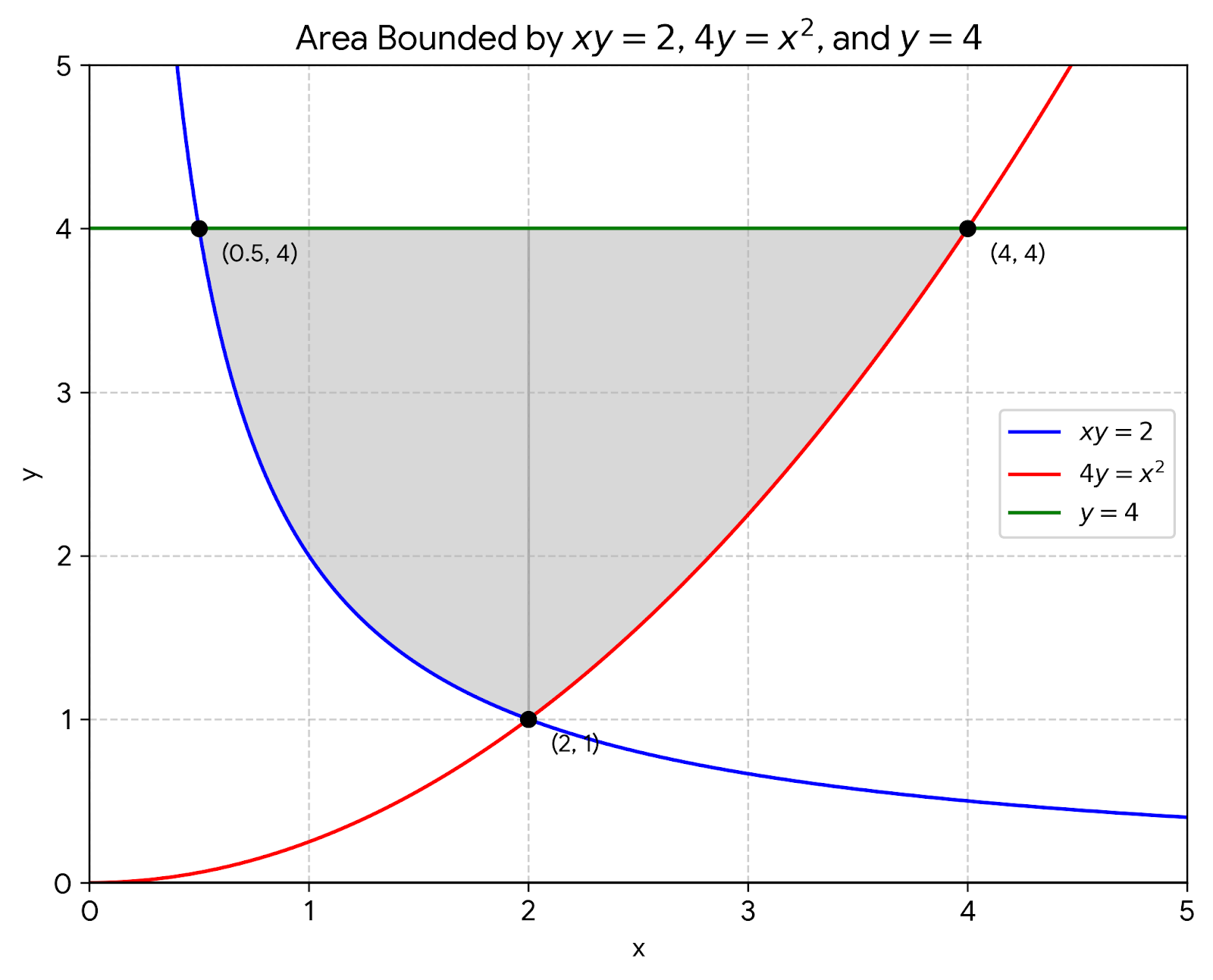
Step 2: Set up the integral

We can integrate with respect to the x-axis or the y-axis. Integrating with respect to the y-axis is much simpler because it only requires evaluating a single integral.

We look at the region from the lowest y-value (y = 1) to the highest y-value (y = 4).

• The right boundary is the parabola: x = 2\sqrt{y}
• The left boundary is the hyperbola: x = \frac{2}{y}

The formula for the area bounded between these curves along the y-axis is:
\text{Area} = \int_{y_1}^{y_2} (x_{\text{right}} - x_{\text{left}}) \, dy

Step 3: Evaluate the integral

Substitute the boundaries and limits into the formula:
\text{Area} = \int_{1}^{4} \left( 2\sqrt{y} - \frac{2}{y} \right) \, dy

Now, integrate term by term:
\text{Area} = 2 \int_{1}^{4} y^{\frac{1}{2}} \, dy - 2 \int_{1}^{4} \frac{1}{y} \, dy
\text{Area} = 2 \left[ \frac{y^{\frac{3}{2}}}{\frac{3}{2}} \right]_{1}^{4} - 2 \big[ \ln|y| \big]_{1}^{4}
\text{Area} = \left[ \frac{4}{3} y^{\frac{3}{2}} \right]_{1}^{4} - 2 \big( \ln(4) - \ln(1) \big)

Evaluate at the limits:
\text{Area} = \frac{4}{3} \big( 4^{\frac{3}{2}} - 1^{\frac{3}{2}} \big) - 2(\ln 4 - 0)

Since 4^{\frac{3}{2}} = (\sqrt{4})^3 = 2^3 = 8:
\text{Area} = \frac{4}{3} (8 - 1) - 2\ln(4)
\text{Area} = \frac{4}{3} (7) - 2\ln(2^2)
\text{Area} = \frac{28}{3} - 4\ln(2)

Final Answer:
The area bounded by the given curves is \frac{28}{3} - 4\ln(2) square units.

Solution:

Step 1: Express the given lines in symmetrical Cartesian form

Let the first line be L_1. The equations are x = 0 and \frac{y}{2} + \frac{z}{3} = 1.
Rewriting the second equation:
\frac{y}{2} = 1 - \frac{z}{3} \implies \frac{y-2}{-2} = \frac{z-0}{3}
Combining this with x=0, the symmetrical form of L_1 is:
\frac{x-0}{0} = \frac{y-2}{-2} = \frac{z-0}{3}
Thus, L_1 passes through the point (x_1, y_1, z_1) = (0, 2, 0) and its direction ratios are a_1, b_1, c_1 = 0, -2, 3.

Let the second line be L_2. The equations are y = 0 and \frac{x}{4} - \frac{z}{3} = 1.
Rewriting the second equation:
\frac{x}{4} = 1 + \frac{z}{3} \implies \frac{x-4}{4} = \frac{z-0}{3}
Combining this with y=0, the symmetrical form of L_2 is:
\frac{x-4}{4} = \frac{y-0}{0} = \frac{z-0}{3}
Thus, L_2 passes through the point (x_2, y_2, z_2) = (4, 0, 0) and its direction ratios are a_2, b_2, c_2 = 4, 0, 3.

Step 2: Find the direction cosines of the line of shortest distance

The line of shortest distance is the common perpendicular to both L_1 and L_2. Let its direction ratios be l, m, n.
Since it is perpendicular to both lines, we have:
0 \cdot l - 2 \cdot m + 3 \cdot n = 0
4 \cdot l + 0 \cdot m + 3 \cdot n = 0

Using cross-multiplication to solve for proportional values of l, m, n:
\frac{l}{(-2)(3) - (0)(3)} = \frac{m}{(3)(4) - (0)(3)} = \frac{n}{(0)(0) - (-2)(4)}
\frac{l}{-6} = \frac{m}{12} = \frac{n}{8}

Dividing the denominators by 2 to simplify, the direction ratios of the shortest distance line are -3, 6, 4.
To convert these direction ratios into direction cosines, we divide by the magnitude \sqrt{(-3)^2 + 6^2 + 4^2} = \sqrt{9 + 36 + 16} = \sqrt{61}.
The direction cosines (l, m, n) of the common perpendicular are:
l = \frac{-3}{\sqrt{61}}, \quad m = \frac{6}{\sqrt{61}}, \quad n = \frac{4}{\sqrt{61}}

Step 3: Calculate the shortest distance using the projection method

The shortest distance (SD) is the length of the projection of the line segment joining the points (0, 2, 0) and (4, 0, 0) onto the common perpendicular. The formula is:
SD = |(x_2 - x_1)l + (y_2 - y_1)m + (z_2 - z_1)n|

Substitute the coordinates of the points and the direction cosines:
SD = \left| (4 - 0)\left(\frac{-3}{\sqrt{61}}\right) + (0 - 2)\left(\frac{6}{\sqrt{61}}\right) + (0 - 0)\left(\frac{4}{\sqrt{61}}\right) \right|
SD = \left| 4\left(\frac{-3}{\sqrt{61}}\right) - 2\left(\frac{6}{\sqrt{61}}\right) + 0 \right|
SD = \left| \frac{-12}{\sqrt{61}} - \frac{12}{\sqrt{61}} \right|
SD = \left| \frac{-24}{\sqrt{61}} \right|

Final Answer:
The shortest distance between the given lines is \frac{24}{\sqrt{61}} units.

Solution:

Step 1: Find the eigenvalues of matrix A

The characteristic equation of A is given by |A - \lambda I| = 0, where I is the identity matrix.
\begin{vmatrix} 2-\lambda & 0 \\ 0 & 1-\lambda \end{vmatrix} = 0
(2-\lambda)(1-\lambda) - (0)(0) = 0

So, the eigenvalues are \lambda_1 = 2 and \lambda_2 = 1.

Step 2: Find the corresponding eigenvectors

For \lambda_1 = 2:
We solve (A - 2I)X = 0
\begin{pmatrix} 2-2 & 0 \\ 0 & 1-2 \end{pmatrix} \begin{pmatrix} x \\ y \end{pmatrix} = \begin{pmatrix} 0 \\ 0 \end{pmatrix}
\begin{pmatrix} 0 & 0 \\ 0 & -1 \end{pmatrix} \begin{pmatrix} x \\ y \end{pmatrix} = \begin{pmatrix} 0 \\ 0 \end{pmatrix}
This gives -y = 0 \implies y = 0. Let x = 1.
The first eigenvector is X_1 = \begin{pmatrix} 1 \\ 0 \end{pmatrix}.

For \lambda_2 = 1:
We solve (A - 1I)X = 0
\begin{pmatrix} 2-1 & 0 \\ 0 & 1-1 \end{pmatrix} \begin{pmatrix} x \\ y \end{pmatrix} = \begin{pmatrix} 0 \\ 0 \end{pmatrix}
\begin{pmatrix} 1 & 0 \\ 0 & 0 \end{pmatrix} \begin{pmatrix} x \\ y \end{pmatrix} = \begin{pmatrix} 0 \\ 0 \end{pmatrix}
This gives x = 0. Let y = 1.
The second eigenvector is X_2 = \begin{pmatrix} 0 \\ 1 \end{pmatrix}.

Step 3: Construct the modal matrix P and diagonal matrix D

The modal matrix P is formed by placing the eigenvectors as columns:
P = \begin{pmatrix} 1 & 0 \\ 0 & 1 \end{pmatrix} = I
Since P is the identity matrix, its inverse P^{-1} is also the identity matrix: P^{-1} = \begin{pmatrix} 1 & 0 \\ 0 & 1 \end{pmatrix}.

The diagonal matrix D is formed by the eigenvalues on the main diagonal:
D = \begin{pmatrix} 2 & 0 \\ 0 & 1 \end{pmatrix}

Step 4: Compute A^{100}

The concept of diagonalization states that A = PDP^{-1}. Therefore, A^n = P D^n P^{-1}.
For n = 100:
A^{100} = P D^{100} P^{-1}

To find D^{100}, we simply raise the diagonal elements to the power of 100:
D^{100} = \begin{pmatrix} 2^{100} & 0 \\ 0 & 1^{100} \end{pmatrix} = \begin{pmatrix} 2^{100} & 0 \\ 0 & 1 \end{pmatrix}

Now, substitute P, D^{100}, and P^{-1} back into the equation:
A^{100} = \begin{pmatrix} 1 & 0 \\ 0 & 1 \end{pmatrix} \begin{pmatrix} 2^{100} & 0 \\ 0 & 1 \end{pmatrix} \begin{pmatrix} 1 & 0 \\ 0 & 1 \end{pmatrix}

Since multiplying by the identity matrix does not change a matrix, we get:
A^{100} = \begin{pmatrix} 2^{100} & 0 \\ 0 & 1 \end{pmatrix}

Final Answer:
A^{100} = \begin{pmatrix} 2^{100} & 0 \\ 0 & 1 \end{pmatrix}

Solution:

Step 1: Expand the integral

First, we multiply the terms in the numerator and split the integral into two separate parts:
I = \int_{0}^{\infty}\frac{x^{8} - x^{16}}{(1+x)^{24}}dx = \int_{0}^{\infty}\frac{x^{8}}{(1+x)^{24}}dx - \int_{0}^{\infty}\frac{x^{16}}{(1+x)^{24}}dx

Step 2: Apply the Beta function definition

The standard property of the Beta function relating to algebraic integrals is:
B(m,n) = \int_{0}^{\infty} \frac{x^{m-1}}{(1+x)^{m+n}}dx

Let’s map our two integrals to this standard form:

• For the first integral: m - 1 = 8 \implies m = 9.
  The denominator power is m + n = 24 \implies 9 + n = 24 \implies n = 15.
  So, \int_{0}^{\infty}\frac{x^{8}}{(1+x)^{24}}dx = B(9, 15).
• For the second integral: m - 1 = 16 \implies m = 17.
  The denominator power is m + n = 24 \implies 17 + n = 24 \implies n = 7.
  So, \int_{0}^{\infty}\frac{x^{16}}{(1+x)^{24}}dx = B(17, 7).

Therefore, the total integral is:
I = B(9, 15) - B(17, 7)

Step 3: Convert to Gamma functions

Using the relationship between Beta and Gamma functions, B(m,n) = \frac{\Gamma(m)\Gamma(n)}{\Gamma(m+n)}, and knowing that for integers \Gamma(n) = (n-1)!:
I = \frac{\Gamma(9)\Gamma(15)}{\Gamma(24)} - \frac{\Gamma(17)\Gamma(7)}{\Gamma(24)}
I = \frac{8! \cdot 14!}{23!} - \frac{16! \cdot 6!}{23!}

Step 4: Factor and simplify

We can factor out the smaller factorials, 6! and 14!, from the numerator:
I = \frac{(8 \times 7 \times 6!) \cdot 14! - (16 \times 15 \times 14!) \cdot 6!}{23!}
I = \frac{6! \cdot 14! \cdot (56 - 240)}{23!}
I = \frac{-184 \cdot 6! \cdot 14!}{23!}

Now, expand 23! down to 14! to cancel it out:
I = \frac{-184 \cdot 6!}{23 \times 22 \times 21 \times 20 \times 19 \times 18 \times 17 \times 16 \times 15}

Calculate the numerator: -184 \times (6 \times 5 \times 4 \times 3 \times 2 \times 1) = -184 \times 720 = -132480.
Notice that in the denominator, the product 23 \times 20 \times 18 \times 16 = 132480.
This allows for a perfect cancellation:
I = \frac{-(23 \times 20 \times 18 \times 16)}{23 \times 22 \times 21 \times 20 \times 19 \times 18 \times 17 \times 16 \times 15}
I = \frac{-1}{22 \times 21 \times 19 \times 17 \times 15}

Multiplying the remaining terms in the denominator:
I = \frac{-1}{2238390}

Final Answer:
The value of the integral is -\frac{1}{2238390}.

Solution:

Step 1: Write down the standard Legendre polynomials

To express a given polynomial in terms of Legendre polynomials, we need the standard formulas for P_n(x) up to the highest power in the function (which is x^4):

Step 2: Express powers of x in terms of P_n(x)

We rearrange the above formulas to solve for x, x^2, x^3, and x^4:

From P_1(x):

From P_2(x):

From P_3(x):

From P_4(x):

Substitute x^2 into this equation:

Step 3: Substitute into the given polynomial f(x)

Given function: f(x) = x^4 + 2x^3 - 6x^2 + 5x - 3

Substitute the expressions we derived:

Step 4: Group like terms and simplify

Now, collect the coefficients for each Legendre polynomial.

For P_4(x):

For P_3(x):

For P_2(x):

For P_1(x):

For P_0(x):

Final Answer:

Putting it all together, the function expressed in terms of Legendre polynomials is:

Solution:

Step 1: Understand the requirements for a basis

To show that a set S = \{u_1, u_2, \dots, u_n\} is a basis for the vector space V, we must formally prove two conditions:

1. S is linearly independent.
2. S spans V (i.e., every vector in V can be written as a linear combination of the vectors in S).

The problem explicitly states that S is a maximal linearly independent set. This inherently satisfies the first condition. Therefore, we only need to prove the second condition: that S spans V.

Step 2: Set up the proof for spanning

Let v be any arbitrary vector in the vector space V. We need to show that v can be expressed as a linear combination of \{u_1, u_2, \dots, u_n\}.

There are two possibilities for the vector v:

• Case 1: v \in S.
  If v is already in the set S (for example, v = u_1), then it can trivially be written as a linear combination: v = 1 \cdot u_1 + 0 \cdot u_2 + \dots + 0 \cdot u_n. Thus, v is in the span of S.
• Case 2: v \notin S.
  This is the main case we must prove.

Step 3: Analyze Case 2 using the maximal property

Assume v \notin S. Let us create a new set S' by adding the vector v to our existing set S:

Since S is defined as the maximal linearly independent set in V, adding any other vector from V to S must destroy its linear independence. Therefore, the new set S' must be linearly dependent.

Step 4: Apply the definition of linear dependence

Because S' is linearly dependent, there exist scalars c_1, c_2, \dots, c_n, a belonging to the underlying field, not all zero, such that their linear combination equals the zero vector:

Now, we must firmly establish that the scalar a cannot be zero.

Proof by contradiction: Suppose a = 0. Then our equation reduces to:

But we already know that the original set S = \{u_1, u_2, \dots, u_n\} is linearly independent. By the definition of linear independence, the only way a linear combination of its elements can equal zero is if all the coefficients are zero. This forces c_1 = c_2 = \dots = c_n = 0.

However, if a = 0 and all c_i = 0, this contradicts our earlier statement that not all scalars are zero (the condition for S' being linearly dependent). Thus, our assumption that a = 0 must be false.

Therefore, we can confidently state that a \neq 0.

Step 5: Express v as a linear combination

Since a \neq 0, we can safely divide by it. Let’s rearrange the equation to solve for v:

Divide the entire equation by a:

Let k_i = -\frac{c_i}{a} represent new scalars. We can rewrite this cleanly as:

Final Conclusion:

This equation proves that any arbitrary vector v \in V can be expressed as a linear combination of the vectors in S. Thus, S spans V. Since S is both linearly independent and spans the vector space V, it formally constitutes a basis for V. Hence Proved.

Solution:

Step 1: Establish the properties of the inverse function

Since f is a one-to-one (injective) and continuous function on an open interval I, it is strictly monotonic. Therefore, its inverse function, which we will denote as g = f^{-1}, exists and is defined on the interval J = f(I).

By the standard theorems of real analysis, the inverse of a continuous and strictly monotonic function on an interval is also continuous. Thus, g is continuous on J.

Step 2: Set up the difference quotient for the derivative of g

We are given y_0 = f(x_0), which means x_0 = g(y_0).

To find the derivative of g at y_0, we must evaluate the following limit:

Let y be an arbitrary point in J such that y \neq y_0. Since f is bijective from I to J, there exists a unique x \in I such that y = f(x).

Because f is one-to-one, y \neq y_0 \implies f(x) \neq f(x_0) \implies x \neq x_0.

Step 3: Substitute variables to transform the limit

Substitute g(y) = x, g(y_0) = x_0, y = f(x), and y_0 = f(x_0) into the difference quotient:

Since x \neq x_0, we can rewrite this fraction by dividing the numerator and the denominator by (x - x_0):

Step 4: Evaluate the limit as y \to y_0

We established in Step 1 that g is continuous at y_0. Therefore, as y \to y_0, g(y) \to g(y_0). This is exactly equivalent to saying as y \to y_0, x \to x_0.

Now, apply the limit to our transformed equation:

Step 5: Apply the definition of the derivative of f

Using the limit laws, the limit of a quotient is the quotient of the limits, provided the limit of the denominator exists and is not zero:

We are given that f is differentiable at x_0, meaning \lim_{x \to x_0} \frac{f(x) - f(x_0)}{x - x_0} = f^{\prime}(x_0). We are also explicitly given that f^{\prime}(x_0) \neq 0, so the division is valid.

Final Conclusion:

Replacing g with f^{-1}, we have proven that the inverse function is differentiable at y_0 and its derivative is:

Hence Proved.

Solution:

Step 1: Define the functions

Let the objective function to be minimized be:
f(x, y, z) = x^2 + y^2 + z^2

Let the given constraints be:
g(x, y, z) = x + y + z - 1 = 0
h(x, y, z) = xyz + 1 = 0

Step 2: Set up the Lagrangian

Using the Lagrange multipliers \lambda and \mu, we construct the Lagrangian function L:
L(x, y, z, \lambda, \mu) = f(x,y,z) + \lambda g(x,y,z) + \mu h(x,y,z)
L = x^2 + y^2 + z^2 + \lambda(x + y + z - 1) + \mu(xyz + 1)

Step 3: Find the partial derivatives

For finding the stationary points, we equate the partial derivatives of L with respect to x, y, z to zero:

\frac{\partial L}{\partial x} = 2x + \lambda + \mu yz = 0 \quad \dots \text{(1)}
\frac{\partial L}{\partial y} = 2y + \lambda + \mu xz = 0 \quad \dots \text{(2)}
\frac{\partial L}{\partial z} = 2z + \lambda + \mu xy = 0 \quad \dots \text{(3)}

Step 4: Solve the system of equations

Subtract equation (2) from equation (1):
(2x - 2y) + \mu(yz - xz) = 0
2(x - y) - \mu z(x - y) = 0 \implies (x - y)(2 - \mu z) = 0

Subtract equation (3) from equation (2):
(2y - 2z) + \mu(xz - xy) = 0
2(y - z) - \mu x(y - z) = 0 \implies (y - z)(2 - \mu x) = 0

Subtract equation (3) from equation (1):
(2x - 2z) + \mu(yz - xy) = 0
2(x - z) - \mu y(x - z) = 0 \implies (x - z)(2 - \mu y) = 0

This gives us a complete system of three factored equations. We have a few cases to analyze based on these factors:

• Case A: All three variables are distinct (x \neq y \neq z)
  If no variables are equal, then to satisfy the equations, we must have \mu z = 2, \mu x = 2, and \mu y = 2. This would mean x = y = z = 2/\mu, which contradicts the assumption that they are distinct. Thus, this case yields no solutions.
• Case B: All three variables are equal (x = y = z)
  Substitute x = y = z into the first constraint: x + x + x = 1 \implies 3x = 1 \implies x = 1/3.
  Now check the second constraint: (1/3)(1/3)(1/3) + 1 = 1/27 + 1 = 28/27 \neq 0.
  Since the second constraint is not satisfied, this case yields no valid points.
• Case C: Two variables are equal, and the third is different
  Without loss of generality, assume x = y and z \neq x.

Step 5: Solve for the specific point (Case C)

Substitute y = x into the first constraint:
x + x + z = 1 \implies z = 1 - 2x

Substitute y = x and z = 1 - 2x into the second constraint:
x \cdot x \cdot (1 - 2x) + 1 = 0
x^2(1 - 2x) + 1 = 0
-2x^3 + x^2 + 1 = 0 \implies 2x^3 - x^2 - 1 = 0

By inspection, x = 1 is a root of this cubic equation because 2(1)^3 - (1)^2 - 1 = 0. Let’s factor out (x - 1):
(x - 1)(2x^2 + x + 1) = 0

The quadratic factor 2x^2 + x + 1 = 0 has a discriminant of \Delta = 1^2 - 4(2)(1) = -7. Since \Delta \lt 0, it has no real roots. Therefore, the only real solution is x = 1.

Using x = 1:
y = x = 1
z = 1 - 2(1) = -1

So, one stationary point is (1, 1, -1). By symmetry, if we had chosen y = z or x = z, we would have found the permutations of this point: (1, -1, 1) and (-1, 1, 1).

Step 6: Confirm the point is a minimum

Geometrically, the objective function f(x,y,z) = x^2 + y^2 + z^2 represents the square of the distance from the origin to a point (x,y,z) on the intersection of the plane x+y+z=1 and the surface xyz=-1.

Because the surface xyz=-1 extends infinitely away from the origin in multiple directions along the plane (for example, if x \to \infty, y \to -\infty, and z \to 0), the distance to the origin is unbounded above. Therefore, a maximum value does not exist. Since the function is bounded below by 0 and must reach an extremum on this closed intersection, the single set of symmetric stationary points we found must represent the absolute minimum distance.

Step 7: Evaluate the minimum value

We substitute any of these stationary points into our objective function f(x,y,z):
f(1, 1, -1) = (1)^2 + (1)^2 + (-1)^2
f(1, 1, -1) = 1 + 1 + 1 = 3

Final Answer:
The minimum value of x^2 + y^2 + z^2 subject to the given constraints is 3.

Solution:

Important Note for Aspirants: There is a classic mathematical typo in the wording of this specific function. The function f(x,y) = \frac{xy}{x^2+y^2} possesses partial derivatives at the origin, but it does NOT possess a directional derivative in EVERY direction. (The classic function that has directional derivatives in all directions but is discontinuous is \frac{x^2y}{x^4+y^2}). If this exact wording appeared in the exam, the best approach is to calculate the directional derivative to show where it fails, prove the partial derivatives exist, and then prove the discontinuity. This demonstrates complete mastery to the examiner.

Step 1: Examine the directional derivatives at (0,0)

Let \vec{u} = (u_1, u_2) = (\cos \theta, \sin \theta) be a unit vector representing an arbitrary direction.

By definition, the directional derivative of f at (0,0) in the direction of \vec{u} is:

This limit only evaluates to a finite number (zero) if \cos\theta\sin\theta = 0, which happens when \theta = 0, \frac{\pi}{2}, \pi, \frac{3\pi}{2} (i.e., along the x and y axes). For any other direction, the limit approaches infinity and does not exist. Thus, we evaluate the partial derivatives specifically.

Step 2: Show that partial derivatives exist at (0,0)

The partial derivative with respect to x is the directional derivative along the x-axis (\theta = 0):

The partial derivative with respect to y is the directional derivative along the y-axis (\theta = \frac{\pi}{2}):

Hence, the partial derivatives exist at the origin and are both equal to 0.

Step 3: Test for continuity at (0,0)

A function is continuous at (0,0) if \lim_{(x,y) \to (0,0)} f(x,y) = f(0,0) = 0. The limit must be the same regardless of the path taken to approach the origin.

Let us approach (0,0) along the straight lines y = mx, where m is the slope.

Final Conclusion:

The value of the limit depends on m. For example, if we approach along y = x (m=1), the limit is \frac{1}{2}. If we approach along y = 2x (m=2), the limit is \frac{2}{5}. Since the limit is not unique and depends on the path of approach, \lim_{(x,y) \to (0,0)} f(x,y) does not exist.

Therefore, f(x,y) is not continuous at (0,0), even though its partial derivatives exist at that point. Hence Proved.

Solution:

Step 1: Identify the nature of the improper integral

Let f(x) = \frac{\log x}{\sqrt{x}}. The point x = 0 is a point of infinite discontinuity because \lim_{x \to 0^+} f(x) = -\infty. Thus, it is an improper integral of the second kind.

Step 2: Prepare for convergence tests (Absolute Convergence)

To use standard comparison tests, the integrand must be strictly positive. For x \in (0, 1), \log x \lt 0, which makes f(x) negative.

We will instead test for absolute convergence by examining the absolute value of the function:

If \int_{0}^{1} |f(x)| dx converges, then the original integral converges absolutely, which guarantees its convergence.

Step 3: Apply the Limit Comparison Test (\mu-Test)

We choose a comparison function of the form g(x) = \frac{1}{x^\mu}.

We need to evaluate the limit L = \lim_{x \to 0^+} \frac{|f(x)|}{g(x)} = \lim_{x \to 0^+} x^\mu |f(x)|:

We want to choose \mu such that this limit evaluates to a finite number (preferably 0) AND the integral of our comparison function g(x) converges. By the p-test for improper integrals of the second kind, \int_{0}^{1} \frac{1}{x^\mu} dx converges if and only if \mu \lt 1.

To ensure the x term pushes the \log x to 0 in our limit, the exponent must be positive, so we also need \mu - \frac{1}{2} \gt 0 \implies \mu \gt \frac{1}{2}.

Let us select \mu = \frac{3}{4}, which safely satisfies \frac{1}{2} \lt \mu \lt 1.

Now, evaluate the limit with \mu = \frac{3}{4}:

Step 4: Evaluate the limit using L’Hôpital’s Rule

Rewrite the expression to apply L’Hôpital’s Rule (transforming it into the \frac{\infty}{\infty} indeterminate form):

Differentiating the numerator and the denominator:

Step 5: Final Conclusion

Since the limit L = 0 (a finite number) and our chosen \mu = \frac{3}{4} is strictly less than 1, the comparison integral \int_{0}^{1} g(x) dx converges.

By the Limit Comparison Test (the \mu-test), the integral \int_{0}^{1} |f(x)| dx also converges.

Because absolute convergence implies ordinary convergence, the given improper integral is convergent.

Solution:

Step 1: Define the ellipsoid and its diameter

Let the standard equation of the ellipsoid be:

A diameter of an ellipsoid is a chord passing through its center. The center of this standard ellipsoid is at the origin (0, 0, 0).

Let P(x_1, y_1, z_1) be one extremity of a diameter. Since the diameter passes through the origin, the other extremity Q will be symmetrically opposite to P across the origin. Thus, the coordinates of Q are (-x_1, -y_1, -z_1).

Step 2: Find the direction cosines of the tangent plane at P

The equation of the tangent plane to the ellipsoid at the point P(x_1, y_1, z_1) is:

The direction ratios of the normal to this tangent plane are proportional to the coefficients of x, y, and z. Let’s call these direction ratios a_1, b_1, c_1:

To find the direction cosines (l_1, m_1, n_1) of this normal, we divide the direction ratios by their magnitude D, where D = \sqrt{\left(\frac{x_1}{a^2}\right)^2 + \left(\frac{y_1}{b^2}\right)^2 + \left(\frac{z_1}{c^2}\right)^2}:

Step 3: Find the direction cosines of the tangent plane at Q

Now, the equation of the tangent plane at the opposite extremity Q(-x_1, -y_1, -z_1) is:

The direction ratios of the normal to this second plane, say a_2, b_2, c_2, are:

Notice that the magnitude of this normal vector is exactly the same value D, because the squares of the negative terms become positive. The direction cosines (l_2, m_2, n_2) for this second tangent plane are:

Step 4: Prove the planes are parallel

Comparing the direction cosines of the two normals, we can clearly see the relationship:

When the direction cosines of two normals are either exactly identical or exact negatives of each other, it means they share the same line of action (they are simply oriented in opposite directions). Because their normal vectors are parallel, the planes to which they are perpendicular must also be parallel.

Final Conclusion:
Hence, it is shown that the tangent planes at the extremities of any diameter of an ellipsoid are always parallel. (Hence Proved)

Solution:

Step 1: Find the images of the new basis vectors under T

We first calculate the transformation of each basis vector in B = \{a_1, a_2, a_3\}.

For a_1 = (1, 0, 1):
T(a_1) = (3(1) + 1, -2(1) + 0, -1(1) + 2(0) + 4(1)) = (4, -2, 3)

For a_2 = (-1, 2, 1):
T(a_2) = (3(-1) + 1, -2(-1) + 2, -1(-1) + 2(2) + 4(1)) = (-2, 4, 9)

For a_3 = (2, 1, 1):
T(a_3) = (3(2) + 1, -2(2) + 1, -1(2) + 2(1) + 4(1)) = (7, -3, 4)

Step 2: Set up the linear combinations

To find the matrix of T, we must express each of these image vectors as a linear combination of the basis vectors a_1, a_2, a_3.

Let (x, y, z) be an arbitrary image vector. We set up the equation:

This generates the following system of linear equations:

1) c_1 - c_2 + 2c_3 = x

2) 2c_2 + c_3 = y

3) c_1 + c_2 + c_3 = z

Step 3: Solve for the scalars by substituting the images

Now, we substitute (x, y, z) with the three image vectors we calculated and solve the resulting 3×3 systems of equations directly.

For T(a_1) = (4, -2, 3):
Substitute x=4, y=-2, z=3:
c_{11} - c_{21} + 2c_{31} = 4
2c_{21} + c_{31} = -2
c_{11} + c_{21} + c_{31} = 3
Solving this system yields: c_{11} = \frac{17}{4}, \quad c_{21} = -\frac{3}{4}, \quad c_{31} = -\frac{2}{4}
Thus, T(a_1) = \frac{17}{4}a_1 - \frac{3}{4}a_2 - \frac{2}{4}a_3

For T(a_2) = (-2, 4, 9):
Substitute x=-2, y=4, z=9:
c_{12} - c_{22} + 2c_{32} = -2
2c_{22} + c_{32} = 4
c_{12} + c_{22} + c_{32} = 9
Solving this system yields: c_{12} = \frac{35}{4}, \quad c_{22} = \frac{15}{4}, \quad c_{32} = -\frac{14}{4}
Thus, T(a_2) = \frac{35}{4}a_1 + \frac{15}{4}a_2 - \frac{14}{4}a_3

For T(a_3) = (7, -3, 4):
Substitute x=7, y=-3, z=4:
c_{13} - c_{23} + 2c_{33} = 7
2c_{23} + c_{33} = -3
c_{13} + c_{23} + c_{33} = 4
Solving this system yields: c_{13} = \frac{22}{4}, \quad c_{23} = -\frac{6}{4}, \quad c_{33} = \frac{0}{4}
Thus, T(a_3) = \frac{22}{4}a_1 - \frac{6}{4}a_2 + \frac{0}{4}a_3

Step 4: Construct the transformation matrix

The matrix of T relative to the basis B is formed by taking the sets of scalars (c_1, c_2, c_3) for each image and placing them as the columns of the matrix:

Final Answer:

Solution:

Step 1: Identify the type of equation and choose a substitution

The given differential equation is of the first order but of a higher degree in p. Equations containing algebraic powers of x, y, and p can often be reduced to Clairaut’s Equation by a suitable substitution.

Let us make the substitution:
X = \frac{1}{x} \quad \text{and} \quad Y = y

Step 2: Transform the derivative p into the new coordinate system

We need to find the new derivative, let’s call it P, where P = \frac{dY}{dX}.
Using the chain rule from calculus, \frac{dY}{dX} = \frac{dY/dx}{dX/dx}.

Differentiate our substitutions with respect to x:
\frac{dY}{dx} = \frac{dy}{dx} = p
\frac{dX}{dx} = \frac{d}{dx}\left(x^{-1}\right) = -x^{-2} = -\frac{1}{x^2}

Now, calculate P:
P = \frac{p}{-1/x^2} = -x^2 p

From this, we extract p to substitute back into the original equation:
p = -\frac{P}{x^2}

Step 3: Substitute X, Y, and P into the original equation

Given equation: x^3 p^2 + x^2 y p + a^3 = 0

Substitute p = -\frac{P}{x^2} and y = Y:
x^3 \left(-\frac{P}{x^2}\right)^2 + x^2 Y \left(-\frac{P}{x^2}\right) + a^3 = 0

Since we defined X = \frac{1}{x}, we substitute X into the equation:
X P^2 - Y P + a^3 = 0

Rearranging this to solve for Y:
Y P = P^2 X + a^3 \implies Y = P X + \frac{a^3}{P}

Step 4: Find the General Solution using Clairaut’s Theorem

Result Used: The transformed equation is exactly in the form of Clairaut’s Equation, which is defined as Y = PX + f(P). According to Clairaut’s theorem, the general solution of such an equation is obtained directly by replacing the derivative P with an arbitrary constant c.

Replacing P with c:
Y = cX + \frac{a^3}{c}

Now, substitute the original variables X = \frac{1}{x} and Y = y back into the equation:
y = \frac{c}{x} + \frac{a^3}{c}

Multiply the entire equation by cx to clear the denominators:
cxy = c^2 + a^3 x
c^2 - (xy)c + a^3 x = 0 \quad \dots \text{(Equation A)}

This is the General Solution.

Step 5: Find the Singular Solution using the c-discriminant

Result Used: The singular solution of a differential equation is the envelope of the family of curves given by its general solution. When the general solution is expressed as a quadratic equation in terms of the constant c (i.e., Ac^2 + Bc + C = 0), the envelope is found by setting the discriminant (B^2 - 4AC) to zero.

From our General Solution (Equation A): c^2 - (xy)c + a^3 x = 0
Here, A = 1, B = -xy, and C = a^3 x.

Set the discriminant to zero:
B^2 - 4AC = 0
(-xy)^2 - 4(1)(a^3 x) = 0
x^2 y^2 - 4a^3 x = 0

Factor out x:
x(xy^2 - 4a^3) = 0

Since our initial substitution was X = \frac{1}{x}, we operate under the domain condition that x \neq 0. Therefore, we can divide by x:
xy^2 - 4a^3 = 0

Final Answer:

• The General Solution is: c^2 - cxy + a^3 x = 0 (where c is an arbitrary constant).
• The Singular Solution is: xy^2 = 4a^3

Solution:

Step 1: Define the vector field V

We are given a scalar function f(x,y,z). The gradient of a scalar function produces a vector field. By definition, V = \nabla f (which is also written as grad f):

Step 2: Prove that \text{curl } V = 0

Formula Used: The curl of a vector field V is defined as the cross product of the del operator (\nabla) and the vector V.

We set this up using a determinant:

Expanding this determinant along the first row (broken down to fit the screen):

Which simplifies to the mixed second-order partial derivatives:

Result Used: Clairaut’s Theorem (or Schwarz’s Theorem). For any scalar function f with continuous second partial derivatives, the order of differentiation does not matter. Thus, the mixed partials are equal (e.g., \frac{\partial^2 f}{\partial x \partial y} = \frac{\partial^2 f}{\partial y \partial x}).

Therefore, each term in the parentheses evaluates to zero:

This proves that the curl of a gradient field is always the zero vector.

Step 3: Prove that \text{div } V \neq 0

Formula Used: The divergence of a vector field V = V_x\hat{i} + V_y\hat{j} + V_z\hat{k} is the dot product of the del operator and the vector V.

Substitute V = \nabla f into the divergence formula:

Performing the dot product (sum of the products of corresponding components):

Result Used: Definition of the Laplacian. The sum of the unmixed second partial derivatives is precisely the definition of the Laplacian operator, denoted as \nabla^2 f.

Therefore, \text{div } V = \nabla^2 f.

Step 4: Final Conclusion

The problem states that f(x,y,z) is a solution to the Poisson equation \nabla^2 f = c, where c is a constant.

By substituting this given condition into our divergence result, we get:

By definition, a Poisson equation is distinct from Laplace’s equation (\nabla^2 f = 0) specifically because the right-hand side is non-zero. Since f satisfies a Poisson equation with constant c, it implies c \neq 0.

Therefore, \text{div } V = c \neq 0.

Hence Proved.

Solution:

Step 1: Find the Complementary Function (C.F.)

The associated homogeneous equation is:

The auxiliary (characteristic) equation is m^2 + 16 = 0, which gives roots m = \pm 4i.

Therefore, the Complementary Function is:

From this, we identify the fundamental solutions:
y_1 = \cos 4x \quad \text{and} \quad y_2 = \sin 4x

Step 2: Compute the Wronskian (W)

The Wronskian of y_1 and y_2 is given by W = y_1 y_2' - y_2 y_1'.

Step 3: Setup Variation of Parameters

Let the Particular Integral (P.I.) be y_p = u(x)y_1 + v(x)y_2, where u and v are unknown functions of x.

The right-hand side of the given differential equation is X = 32 \sec 2x.

The formulas for u and v are:

Step 4: Evaluate the integral for u

Using the double angle identity \sin 4x = 2\sin 2x \cos 2x:

Step 5: Evaluate the integral for v

Using the double angle identity \cos 4x = 2\cos^2 2x - 1:

Step 6: Construct the Particular Integral (P.I.)

Substitute u and v back into y_p:

Using the trigonometric identity \cos(A - B) = \cos A \cos B + \sin A \sin B, we simplify the first term:

Step 7: Final General Solution

The complete general solution is the sum of the Complementary Function and the Particular Integral: y = y_c + y_p.

Final Answer:

The general solution is y = C_1 \cos 4x + C_2 \sin 4x + 8\cos 2x - 4\sin 4x \log|\sec 2x + \tan 2x|, where C_1 and C_2 are arbitrary constants.

Solution:

Step 1: Transform into a linear equation with constant coefficients

Let x = e^t, which implies t = \log x. Let D = \frac{d}{dt}. The standard substitutions for a Cauchy-Euler equation are:

• x \frac{dy}{dx} = Dy
• x^2 \frac{d^2y}{dx^2} = D(D-1)y
• x^3 \frac{d^3y}{dx^3} = D(D-1)(D-2)y

Substituting these into the original equation:

Step 2: Find the Complementary Function (C.F.)

The auxiliary equation is m^3 - m^2 + 2 = 0. By inspection, m = -1 is a root (-1 - 1 + 2 = 0). Dividing by (m+1):

The roots are m_1 = -1 and m = \frac{2 \pm \sqrt{4-8}}{2} = 1 \pm i.

Thus, the C.F. in terms of t is:

Converting back to x (e^t=x, t=\log x):

Step 3: Find the Particular Integral (P.I.)

For 10e^t (replace D with 1):
\frac{10e^t}{1-1+2} = 5e^t = 5x

For 10e^{-t} (replace D with -1):
\frac{10e^{-t}}{(-1)^3 - (-1)^2 + 2} = \frac{10e^{-t}}{-1 - 1 + 2} = \frac{10e^{-t}}{0}

Since we have a zero denominator, multiply by t and differentiate the operator D^3-D^2+2 to get 3D^2-2D:

Step 4: Final General Solution

Final Answer:
The general solution is y = \frac{C_1 + 2\log x}{x} + x(C_2 \cos(\log x) + C_3 \sin(\log x)) + 5x.

Solution:

Step 1: Determine the angles between the forces

Let the three forces be P, Q, and R.

• Angle between P and Q is 120^{\circ}.
• Angle between Q and R is 150^{\circ}.

Since the sum of angles around a point is 360^{\circ}, the angle between the third force R and the first force P is:

Step 2: Apply Lami’s Theorem

Result Used: Lami’s Theorem. If three forces acting on a particle are in equilibrium, each force is proportional to the sine of the angle between the other two forces.

Where:

• \alpha is the angle between Q and R = 150^{\circ}
• \beta is the angle between P and R = 90^{\circ}
• \gamma is the angle between P and Q = 120^{\circ}

Step 3: Calculate the ratios

Substituting the sine values:

• \sin 150^{\circ} = \sin(180^{\circ} - 30^{\circ}) = \sin 30^{\circ} = \frac{1}{2}
• \sin 90^{\circ} = 1
• \sin 120^{\circ} = \sin(180^{\circ} - 60^{\circ}) = \sin 60^{\circ} = \frac{\sqrt{3}}{2}

The proportion is:

Multiply all terms by 2 to clear the fractions:

Final Answer:
The ratio between the magnitudes of the forces P : Q : R is 1 : 2 : \sqrt{3}.

Solution:

Step 1: Velocity Proportionality

Let v_r = \dot{r} and v_\theta = r\dot{\theta}. Given v_r = k v_\theta:

Step 2: Acceleration Proportionality

Given radial acceleration a_r = \ddot{r} - r\dot{\theta}^2 and transverse acceleration a_\theta = 2\dot{r}\dot{\theta} + r\ddot{\theta}. Given a_r = k a_\theta:

Step 3: Rigorous Derivation

Differentiate \dot{\theta} = \frac{\dot{r}}{kr} to find \ddot{\theta}:

Substitute \dot{\theta} and \ddot{\theta} into equation (2):

Subtracting \ddot{r} from both sides yields -\frac{\dot{r}^2}{k^2r} = \frac{\dot{r}^2}{r}. This requires \dot{r}^2 = 0 or k^2 = -1, implying the particle must follow \dot{r} = \lambda r for the motion to satisfy the proportionality constant.

Step 4: Proving the Power Law

Integrating \dot{r} = \lambda r gives r = r_0 e^{\lambda t}. Consequently, \dot{\theta} = \frac{\lambda r}{kr} = \frac{\lambda}{k} = \omega (constant angular velocity).

The total velocity magnitude v is:

Since \sqrt{\lambda^2 + \omega^2} is a constant A, we have v = A \cdot r^1.

Final Answer:
We have proven that under the given proportionality constraints, v is directly proportional to r (i.e., v \propto r^1). Thus, the velocity varies as a power of the radius vector.

Solution:

Step 1: Compute the Gradient Vector (\nabla f)

The gradient is defined as \nabla f = \frac{\partial f}{\partial x}\hat{i} + \frac{\partial f}{\partial y}\hat{j} + \frac{\partial f}{\partial z}\hat{k}.

Step 2: Evaluate \nabla f at the point (3, 1, -2)

Substitute x=3, y=1, z=-2:

Thus, \nabla f(3, 1, -2) = 96\hat{i} + 288\hat{j} - 288\hat{k}.

Step 3: Determine the Direction of Maximum Increase

The directional derivative is maximum in the direction of the gradient vector. We can simplify this direction by dividing by the common factor 96:

Step 4: Determine the Magnitude of the Maximum Directional Derivative

The maximum value of the directional derivative is the magnitude of the gradient vector |\nabla f|:

Final Answer:
The maximum directional derivative is in the direction of \hat{i} + 3\hat{j} - 3\hat{k} (or the unit vector \frac{1}{\sqrt{19}}(\hat{i} + 3\hat{j} - 3\hat{k})), and its magnitude is 96\sqrt{19}.

Solution:

Step 1: Define the given conditions

A vector field is called irrotational if its curl is equal to the zero vector. Since we are given that \overline{f} and \overline{g} are irrotational, we have:

Step 2: State the required vector identity

Formula Used: To find the divergence of a cross product of two vector fields, we use the standard vector calculus identity:

Step 3: Apply the identity to \overline{f} \times \overline{g}

Substitute \overline{A} = \overline{f} and \overline{B} = \overline{g} into the identity:

Now, substitute the irrotational conditions from Step 1 (\nabla \times \overline{f} = \mathbf{0} and \nabla \times \overline{g} = \mathbf{0}):

Step 4: Final Conclusion

Result Used: A vector field is called solenoidal if its divergence is zero.

Since we have mathematically proven that the divergence of \overline{f} \times \overline{g} is exactly zero (\nabla \cdot (\overline{f} \times \overline{g}) = 0), the resulting vector field must be solenoidal.

Final Answer:

Hence, it is shown that if \overline{f} and \overline{g} are irrotational, then \overline{f} \times \overline{g} is solenoidal.

Solution:

Step 1: Prepare the equation for transformation

The given differential equation is:

Multiply the entire equation by x to bring it closer to the standard Cauchy-Euler or Bessel structure:

Step 2: Apply the substitution y = x^k u

To eliminate the unwanted coefficient in the first derivative term, we use the substitution y = x^k u, where u is a function of x.

Differentiating y with respect to x:

Substitute these into Equation 1:

Divide the entire equation by x^k:

Combine the like terms for u' and u:

Step 3: Transform into Bessel’s Standard Form

Result Used: The standard form of Bessel’s differential equation of order n is x^2 u'' + x u' + (x^2 - n^2)u = 0.

To match the coefficient of xu' to 1, we must set:

Substitute k = -1/2 into Equation 2. The constant term k^2 + k becomes (-1/2)^2 - 1/2 = 1/4 - 1/2 = -1/4.

Step 4: Scale the independent variable

The term \frac{1}{2}x^2 prevents this from being the exact standard form. Let z = \frac{x}{\sqrt{2}}, which means x = \sqrt{2}z and x^2 = 2z^2.

Using the chain rule, the operators change as follows:

Substitute these into our modified equation:

Step 5: Write the solution in terms of Bessel Functions

This is now exactly Bessel’s equation with order n^2 = 1/4 \implies n = 1/2.

The general solution for u(z) when n is not an integer is a linear combination of the Bessel functions of the first kind J_n and J_{-n}:

Substitute back z = \frac{x}{\sqrt{2}}:

Finally, substitute back into our original transformation y = x^k u = x^{-1/2} u = \frac{1}{\sqrt{x}} u:

Final Answer:

The general solution to the differential equation in terms of Bessel functions is:

(Where C_1 and C_2 are arbitrary constants).

Solution:

Step 1: Compute the derivatives of the proposed solution

We are given the proposed solution y = cx^2 + x + 3, where c is a constant.

First derivative: \frac{dy}{dx} = 2cx + 1

Second derivative: \frac{d^2y}{dx^2} = 2c

Step 2: Verify that it satisfies the differential equation

Substitute y, y', and y'' into the Left Hand Side (LHS) of the given differential equation x^2 y'' - 2xy' + 2y = 6:

Expand the terms:

Group the terms by powers of x:

Since LHS = RHS (6 = 6), the function satisfies the differential equation for all real x.

Step 3: Verify the Initial Conditions

Apply the initial condition y(0) = 3:

This condition is satisfied regardless of the value of c.

Apply the initial condition y'(0) = 1:

This condition is also satisfied regardless of the value of c.

Step 4: Prove Non-Uniqueness

Because the initial conditions y(0)=3 and y'(0)=1 do not place any restriction on the constant c, c can be any arbitrary real number.

For example:

• If c = 1, y = x^2 + x + 3 is a solution.
• If c = 5, y = 5x^2 + x + 3 is a solution.
• If c = 0, y = x + 3 is a solution.

Since there are infinitely many valid solutions for the exact same initial value problem, the solution is not unique.

(Theoretical Justification for Mains Exam): The standard Existence and Uniqueness Theorem (Picard-Lindelöf) requires the differential equation to be written in standard form y'' + P(x)y' + Q(x)y = f(x). Dividing our equation by x^2 gives P(x) = -\frac{2}{x} and Q(x) = \frac{2}{x^2}. Both of these coefficients are discontinuous (singular) at x = 0. Because the initial conditions are given exactly at this singular point x = 0, the fundamental theorem of uniqueness does not apply, allowing for multiple solutions.